

The 1st International Conference on Safety and Public Health
Más datosTo understand the spatial pattern of dengue fever (DF) patients’ survival and investigated factors influencing DF patients’ survival.
MethodA Bayesian spatial survival method via a conditional autoregressive approach was used to analyze the factors that influence DF patients’ survival in 14 sub-districts from January 2015 to May 2017 in Makassar city, Indonesia. Bayesian spatial and a non-spatial model were compared by using deviance information criterion.
ResultsThe spatial model was more suitable than a non-spatial model. Under the Bayesian spatial model, there was a substantive relationship between age, grade and DF patients’ survival time.
ConclusionsThe relative risk map and related factors of DF patients’ survival can indicate the health policy makers to give special attention to the high risk areas in order to faster and more targeted treatment.
Dengue fever (DF) is a disease that often causes outbreaks or epidemics. The recent report from the World Health Organization1 reported that globally, there has been a significant increase in the number of DF every year. Indeed, Indonesia has the most cases of DF disease in Southeast Asia region with more than 129,650 people infected with the virus in 2015.2 Makassar city is one of the areas in Indonesia that has DF virus each year. There is a real need to increase efforts to prevent transmission of the disease and reduce the mortality rate.
Efforts to reduce the death rate from DF virus can be either preventive or curative. An example of a preventive method is raising awareness and a healthy lifestyle to reduce the incidence and spread of DF.3 An example of a curative method is providing the right medical treatment to patients. Here, the issue of survival of patients with DF becomes important to investigate.
Survival time of patients with DF disease can be influenced by many factors. So far in the literature, in general, the factors can be grouped into two major themes. The first theme is associated with physical or biological characteristics of DF patients such as age, gender, etc.1 The second theme covers a number of non-biological factors such as location, local conditions, rainfall, socio-economic conditions and therapy or treatment given to patients with DF.4-7
Survival data are commonly analyzed using proportional hazards regression.8–10 However, this method is based on a relatively simple model and it does not allow the incorporation of external information such as survival spatial information. Bayesian approaches to modelling and analysis of DF have become increasingly popular over the last decade. For example, Honorato et al.11 investigated cases of DF which were spatially distributed in Brazil using a Bayesian spatial hierarchical model using conditional autoregressive (CAR) prior. Lowe et al.12 used a general spatio-temporal mixed model with a Bayesian framework taking into account geographical and temporal resolution to evaluate the spread of DF in Brazil Southeast. Furthermore, Jaya et al.13 used a Bayesian spatial approach to model and map the DF cases in Bandung, Indonesia.
As noted above, most of this literature focuses on incidence and there are fewer papers on DF survival. The literature on spatial modelling of DF survival is even more sparse and limited to small-scale studies.14–18 For example, Thamrin and Taufik14 used multilevel survival to study DF survival. Aswi et al.18 considered DF survival in a single hospital in Makassar using Bayesian Weibull survival and a semiparametric Cox proportional hazards model. In this study, a Bayesian spatial survival method via a CAR approach was used to analyze DF patients’ survival, and to investigate factors that influence DF patients’ survival. This is investigated through a DF patients’ survival in Makassar, Indonesia.
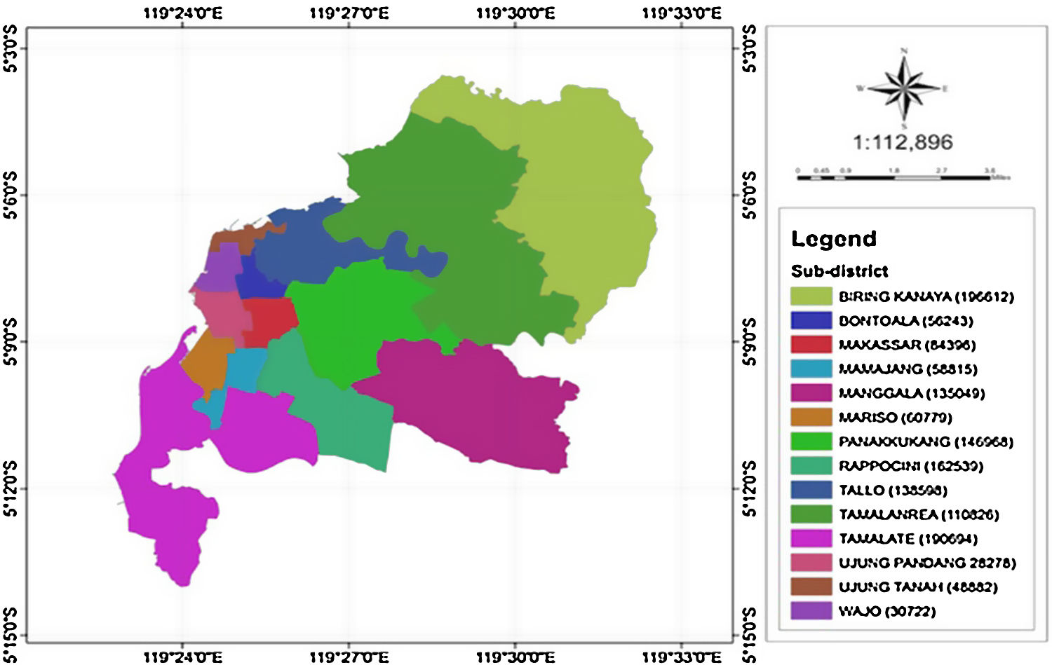
MethodsStudy area and source of dataMakassar is the most populous city in South Sulawesi or even in the eastern part of Indonesia.19 Makassar city consists of 14 sub-districts with 143 villages in these sub-districts (Figure 1).20

Data used were collected from four big hospitals in Makassar city, that is, Dr. Wahidin Sudirohusodo, Labuang Baji, Pelamonia, and Haji Hospitals. In this dataset, the variables used were sex, haematocrit, leukocyte, haemoglobin, thrombocyte, level severity of DF type (grade), age, survival time, and address of DF patients. The number of patients diagnosed with DF were treated in these hospitals, in the period of January 2015 to May 2017 is 934.
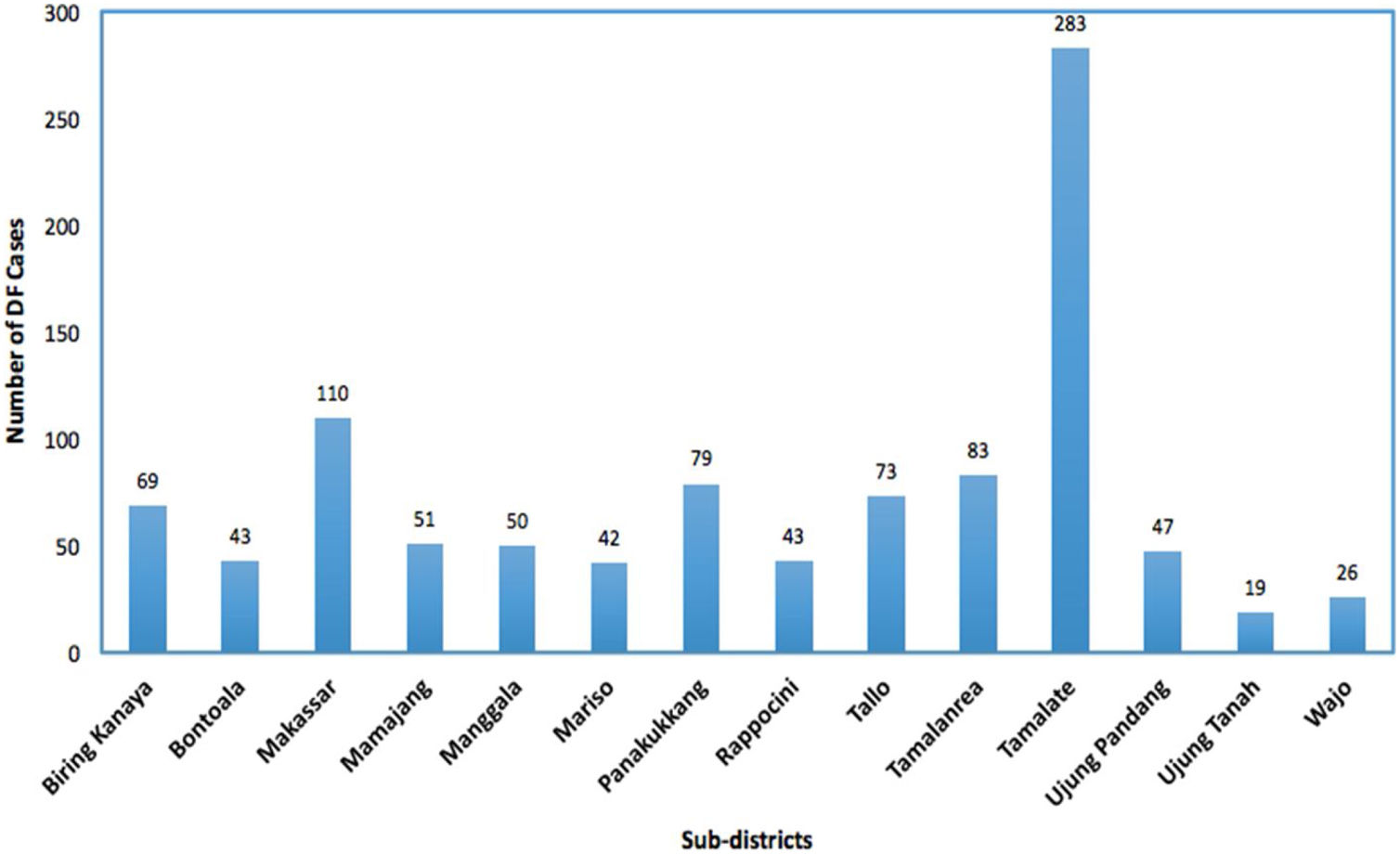
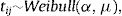
In our models, the survival response variable tij is defined as the number of days that a patient stayed in the hospital until they recovered or got consent to leave the hospital or death. The DF patients self-discharge or transfer to another hospital and still alive at the end of the study period were treated as ‘censored’. The DF incidence rates, which is the number of cases per 10,000 people per year, for each sub-district from the four big hospitals in Makassar city are presented in Figure 2. Data on population numbers for the same time period were collected from the Central Bureau of Statistics of Makassar city, Indonesia.19 The population size was used to calculate and to map the hazard rate.
Spatial survival model
Following the description in Banerjee et al.,17 let tij be the response described in the previous section, namely time to recovery for subject j in sub-district i, j=1,2,…,ni, i=1,2,…,l. Let xij be the corresponding vector of individual-specific covariates. Assume a proportional hazard h(tij;xij) that follows a Weibull distribution with h0(tij)=ρtijρ−1 as follows:
h0(tij) represents a baseline hazard. The exponential term involving the covariates affect the baseline hazard multiplicatively. Here, ρ is the shape parameter of the baseline hazard and the vector β contains the intercept for the baseline hazard. The parameter ρ represents monotonicity of the hazard rate in the Weibull mode,21 where ρ=1 represents a constant hazard rate, and ρ>1 and ρ<1 indicate that the hazard will increase and decrease monotonically with time, respectively. Since Wi=log ωi, in the frailty setting,22 Eq. (1) is extended to:

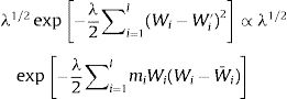
Wi is the sub-district-specific frailty term with distribution:
where log (μ)=β0+βx. CAR denotes a conditionally autoregressive structure Wi|Wi′≠i∼N(W¯i,1/λmi)17,22 and λ is the CAR parameter in Eq. (3) which states thewhere i adj i′ denotes regions i′ that are adjacent to region i, W¯i is the average of the Wi≠i′ that are adjacent to Wi, and mi is the number of these adjacencies.
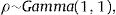
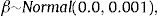

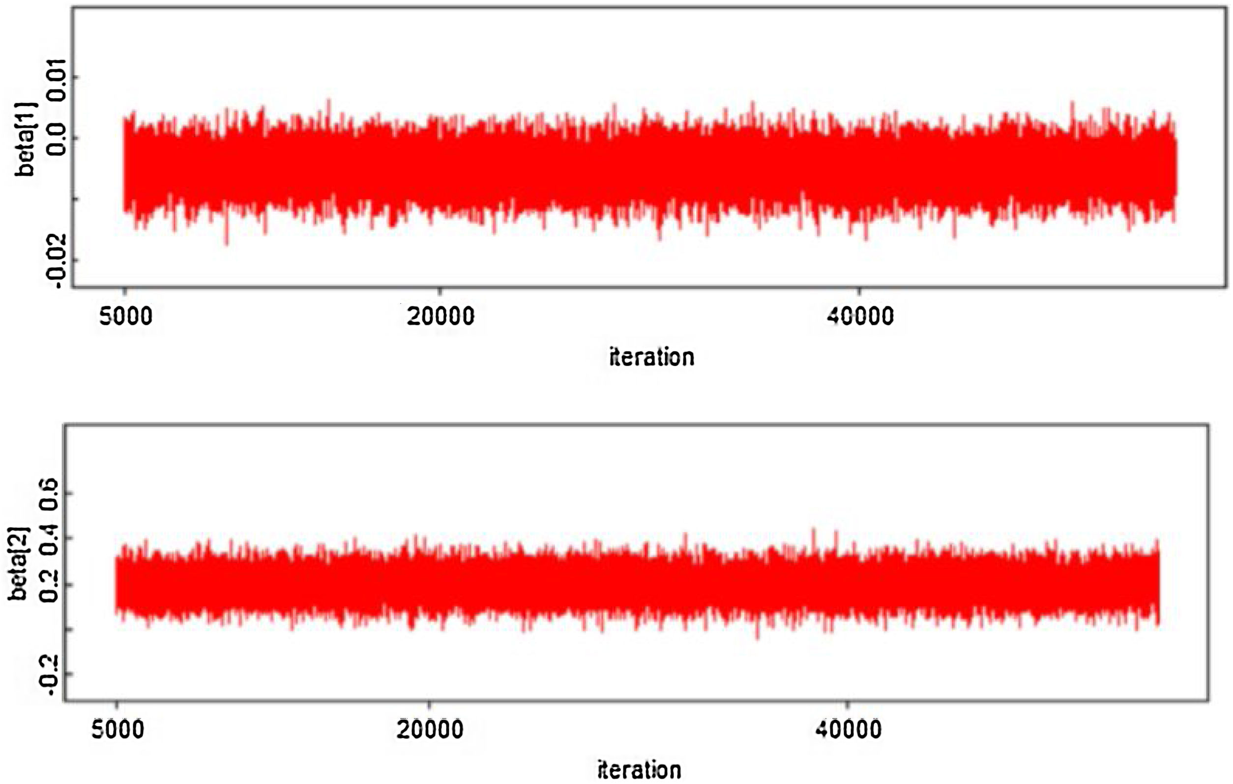
To complete the Bayesian model specification in Eq. (4), we use prior distributions on ρ, β and σ2. We use a gamma hyperprior distribution for λ. With this parameter, the gamma distribution has mean 1 and the variance 1; see Banerjee et al.17 In this paper, we include both spatial and non-spatial frailties.17 Non-spatial frailties means that the model has an unstructured frailty term, expressed as independently and identically distributed (i.i.d) N(0,σ2). The model was fitted using the OpenBUGS software.23 The MCMC algorithm was run with 150,000 iterations, discarding 10,000 as burn-in. Monitoring MCMC convergence was done through trace plots, autocorrelation plots, and plots of the posterior distributions of the model parameters.
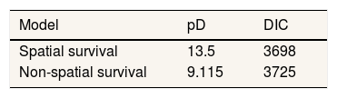
Goodness of fit measures were used to test whether a spatial survival model adequately represents the data. The deviance information criterion (DIC)24 is one of the criteria in evaluating the best model for several data sets using the Bayesian approach. A model is more suitable when it has the smallest DIC.24
ResultsThe model was fitted to DF survival dataset as described in Section “Spatial Survival Model”. By using the different set of starting values, the chain was run. Convergence can be assessed whether it has been achieved or not through the MCMC chain. The results of the hazard rates obtained from Eq. (2) were mapped using the Map tool R version 4.0.2 package.
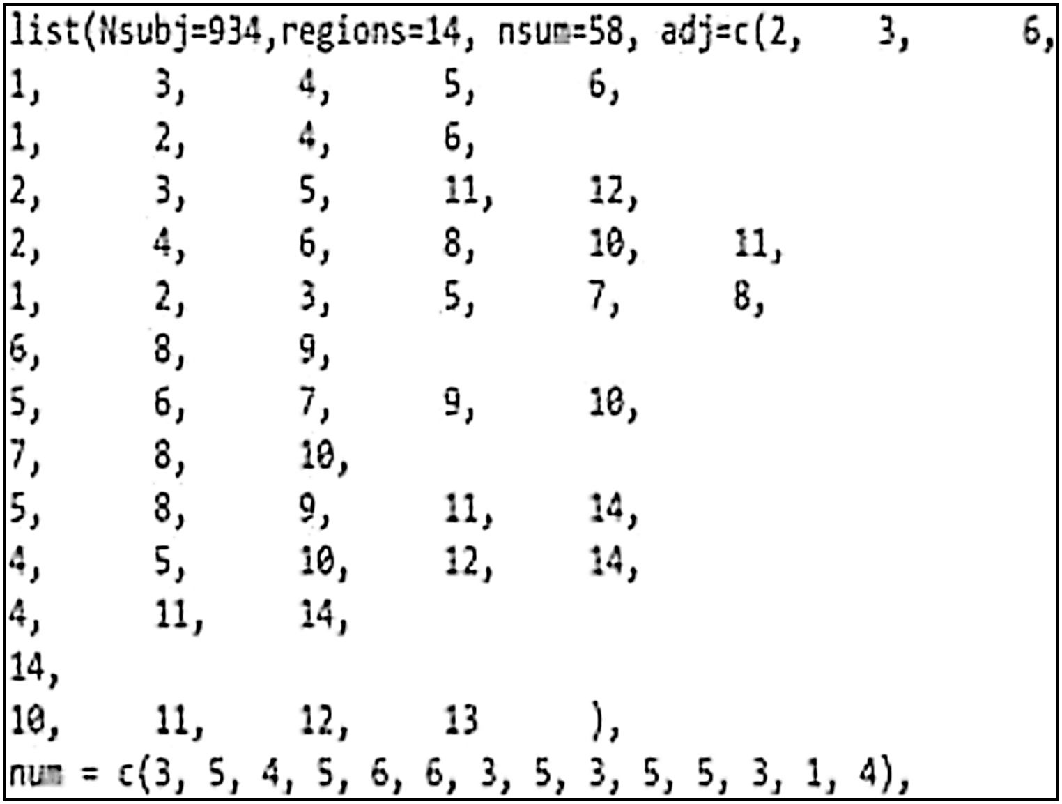
According to Figure 1, the city of Makassar is divided into 14 sub-districts so a spatial weights matrix of queen contiguity order one of 14×14 was formed. The corresponding adjacency matrix for Makassar city, Indonesia is shown in Figure 3. The Weibull assumption for the survival time was assessed by plotting log[−log(S(t))] versus log(t), where the survival probability S(t) was obtained using Kaplan–Meier estimation and t is the survival time. The Weibull distribution was indicated by a straight line plot. This assumption was also verified by application of the Mann test (if Fapproximation=0.784<Fcriterion=1.17 at the 5% level, then the null hypothesis is accepted). The Weibull distribution was thus considered to be appropriate for these data.

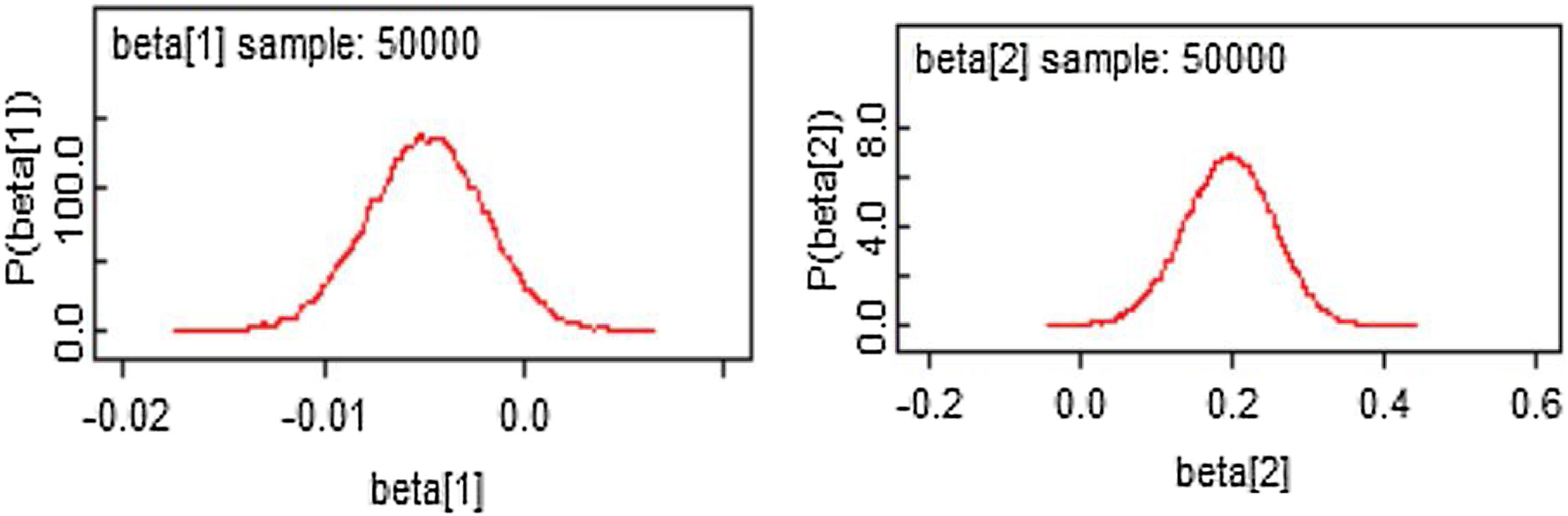
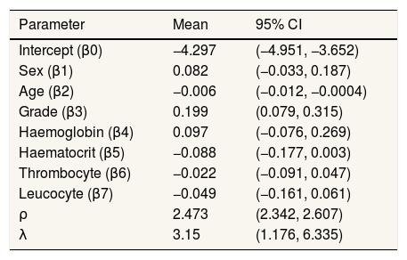
From Figures 4 and 5, the MCMC outputs for the significant parameters of the model in the form of posterior density and trace plots show a well-behaved and fast mixing process. The posterior estimates of parameters and corresponding 95% confidence intervals (CI) are presented in Table 1. It can be inferred that age and grade substantially describe patients’ survival times. The variables age and grade both have a negative effect on the expected survival time. For example, an increase of one year in patient's age increased the hazard at DF survival by exp(−0.006)=0.994 days.


Summary of posterior estimated parameters for spatial survival for DF survival data.
| Parameter | Mean | 95% CI |
|---|---|---|
| Intercept (β0) | −4.297 | (−4.951, −3.652) |
| Sex (β1) | 0.082 | (−0.033, 0.187) |
| Age (β2) | −0.006 | (−0.012, −0.0004) |
| Grade (β3) | 0.199 | (0.079, 0.315) |
| Haemoglobin (β4) | 0.097 | (−0.076, 0.269) |
| Haematocrit (β5) | −0.088 | (−0.177, 0.003) |
| Thrombocyte (β6) | −0.022 | (−0.091, 0.047) |
| Leucocyte (β7) | −0.049 | (−0.161, 0.061) |
| ρ | 2.473 | (2.342, 2.607) |
| λ | 3.15 | (1.176, 6.335) |
Table 2 provides a summary of model fit with a corresponding non-spatial survival model as a comparison. In the latter, Eq. (3) is replaced by Wi∼N(0,σ2). The spatial model is more suitable for these data. This is indicated by the larger size of the effective parameter pD and the smaller value of DIC.
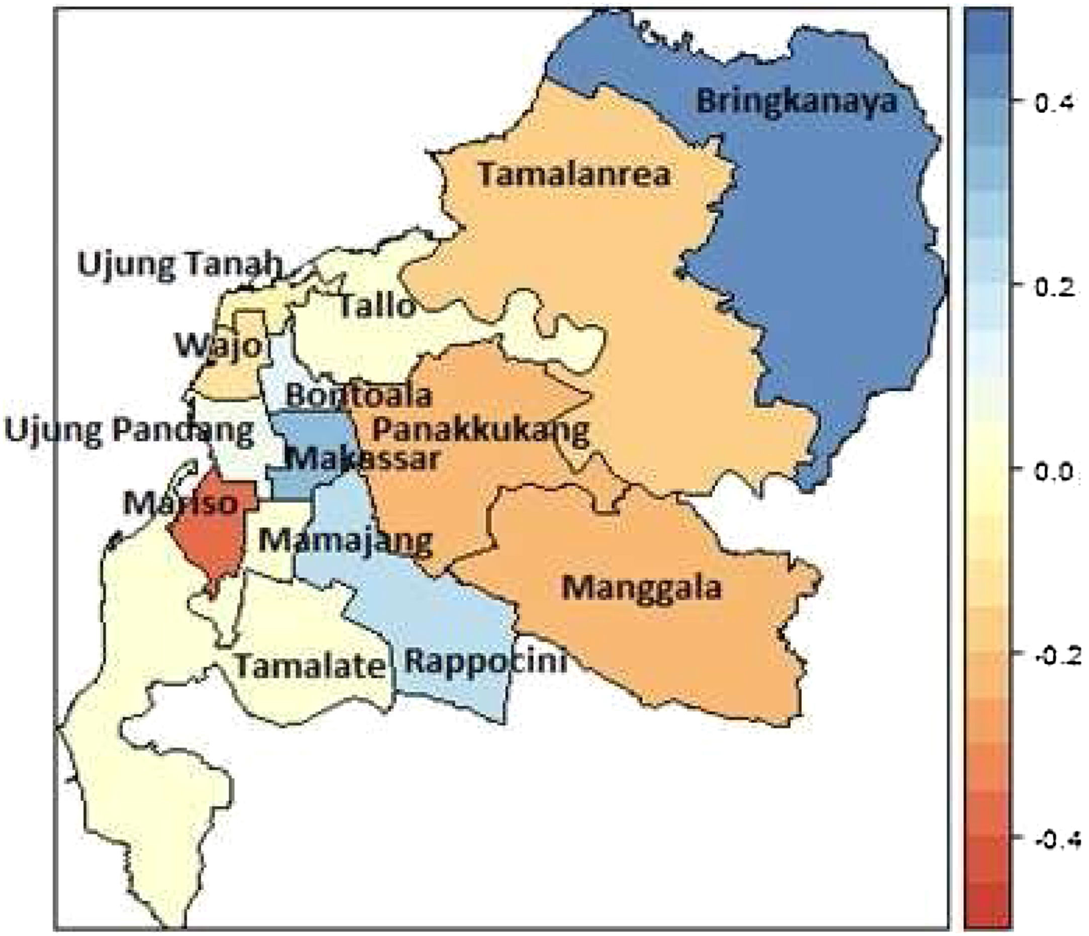
The mapped summary of the posterior mean survival times per sub-district is shown in Figure 6. The results indicate that regional sub-districts located around urban centres, namely Mariso had the lowest hazard rate. The constant hazard rates occurred in the sub-districts Manggala, Panakkukang, Bontoala, Rappocini, Tamalanrea, and Wajo. The higher hazard rate of DF patients occurred in the sub-districts Biringkanaya, Makassar and Mamajang.

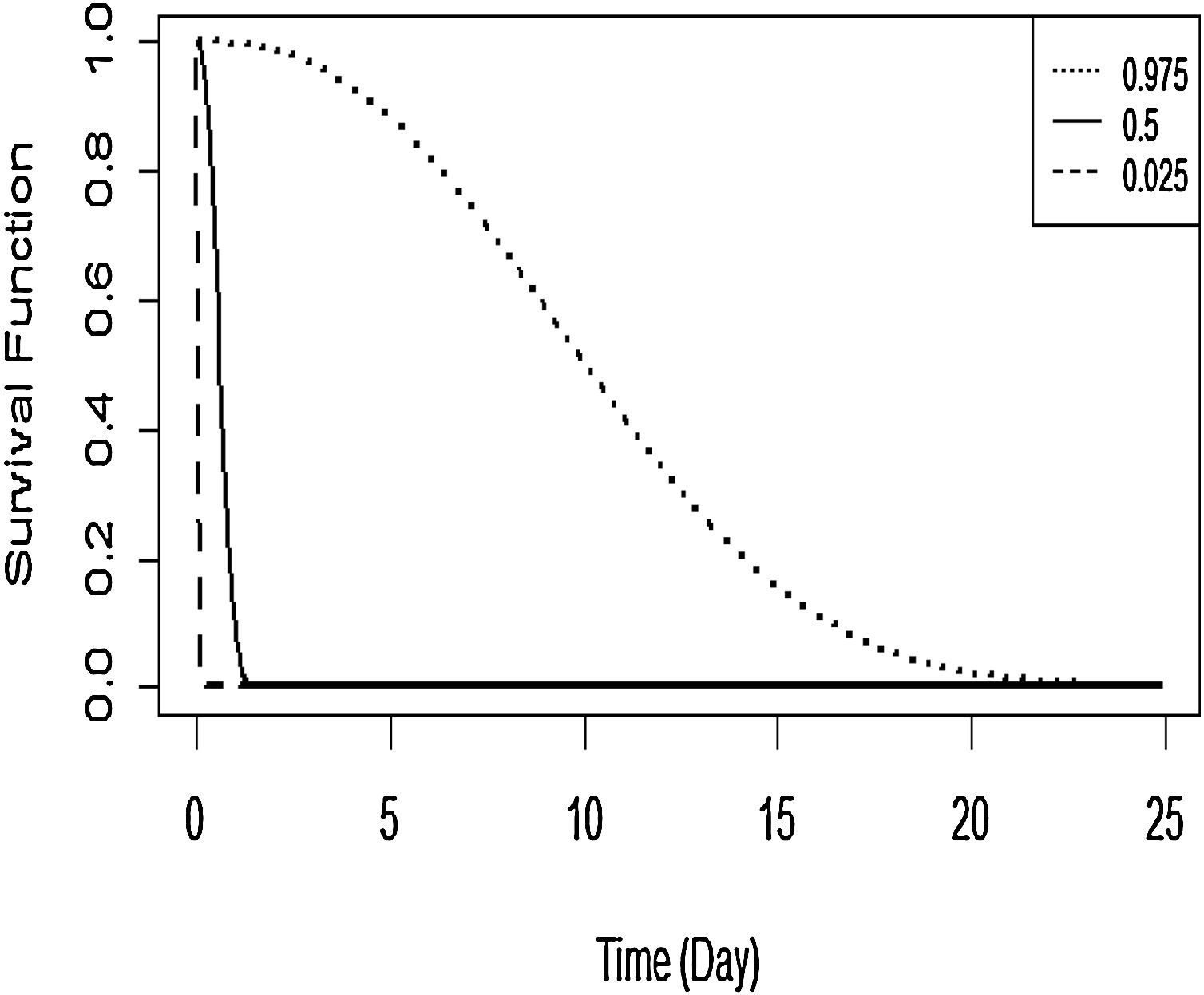
The Kaplan–Meier curve for DF survival with covariates age and grade is shown in Figure 7. The covariates were established for survival time in the first patient for DF. The probability of survival for this first patient is predicted to fall fairly rapidly towards 0.10 when the survival time is about 2 days, then declines very slowly thereafter.
Discussion
We have presented the modelling of the spatial correlated survival data in this paper. To estimate spatial survival with a CAR model, a Bayesian model via a MCMC computational technique was used. The case study used the survival times of DF patients from hospitals in Makassar, Indonesia for the period 2015–2017 with covariates.
Overall, the results of this study indicated that age and grade factors appear to influence the number of days of patients hospitalised with DF until they got recovery or were allowed to go home. The prediction of DF patients’ survival time based on influencing variables is also illustrated. This suggests that when the survival time is about 2 days, the probability of patient's survival time drops fairly rapidly towards 0.10 and decays very slowly thereafter. Mariso had the lowest hazard rate while Biringkanaya had the highest hazard rate, fooled by Makassar and Mamajang. These districts are the potential regions to target for health policy intervention in high risk areas and for more targeted, efficient allocation of the relevant resources. Notwithstanding this, further investigation is needed in order to consider socio economic, temperature, and humidity effects in modelling the survival factors.5–7,12 The flexibility of the Bayesian spatial survival models invites extensions to more complicated scenarios such as a spatial clustering6 and spatial-temporal model.5,25
ConclusionsThe relative risk map and related factors of DF patients’ survival can indicate the health policy makers to give special attention to the high risk areas in order to faster and more targeted treatment.
Authorship contributionsSAT contributed to the concept and design of the study, carried out statistical analysis and wrote manuscripts. AS and KM interpreted the data, analyzed and wrote the manuscript. AKJ carried out the statistical analysis and AN collects the necessary data. All authors read and approved the final manuscript.
Conflicts of interestThe authors declare that there is no conflict of interests.
The first author acknowledges the Ministry of Research, Technology and Higher Education of Indonesia for providing funding for this research through Grant PDUPT Hasanuddin University in 2018 with the number 1623/UN4.21/PL.00.00/2018. The authors acknowledge Dr. Wahidin Sudirohusodo, Labuang Baji, Pelamonia, and Haji Hospitals, South Sulawesi Province for providing the DF dataset.
Peer-review under responsibility of the scientific committee of the 1st International Conference on Safety and Public Health (ICOS-PH 2020). Full-text and the content of it is under responsibility of authors of the article.