




This study provides an introductory tutorial on conducting a simplified cost-utility analysis of a new treatment for a generic cariovascular disease, combining discrete event simulation (DES) and real-world data (RWD). To help readers understand the proposal, we present an application of this approach to a RWD database, along with files containing its implementation in Excel and R and the explanation in Spanish in the Supplementary material.
MethodThis dataset was used to calculate quality-adjusted life years (QALY) and costs for each individual in the observed alternative (standard of care) by combining longitudinal and survival data. Simulated alternative (counterfactual) results were obtained by adding hazard ratios (HR) from published randomised clinical trials to the parametric survival analysis within a discrete event simulation (DES) model. Bootstrapping allowed to assess uncertainty. Life expectancy was estimated using parametric survival analysis in order to extend the analysis to the patient's death.
ResultsThe exercise files in Excel and R are available in the OSF repository (https://osf.io/gyuq9/overview?view_only=748bc600f59646f1b144e21458c50a42). These outline the steps for calculating the QALYs and costs for the standard and new alternatives based on the dataset. The incremental cost-effectiveness ratio is then calculated and the uncertainty of the result analysed using the cost-effectiveness plot and acceptability curve obtained via bootstrapping.
ConclusionsCombining real-world data and DES can enable cost-utility studies to be conducted, thus streamlining the process of economic evaluation. In order to apply this proposal to research studies, additional tools are required, such as probabilistic sensitivity analysis.
Este estudio ofrece un tutorial introductorio sobre cómo realizar un análisis simplificado de coste-utilidad de un nuevo tratamiento para una enfermedad cardiovascular genérica, combinando la simulación de eventos discretos (SED) y datos del mundo real (RWD). Presentamos la aplicación de una base de datos de RWD, junto con archivos que contienen su implementación en Excel y R, así como la explicación en español en el material complementario.
MétodoSe calcularon los años de vida ajustados por calidad (AVAC) y los costes para cada individuo en la alternativa observada (tratamiento estándar) mediante la combinación de datos longitudinales y de supervivencia. Los resultados de la alternativa simulada (contrafactual) se obtuvieron añadiendo las razones de riesgo de ensayos clínicos publicados dentro de un modelo de simulación de eventos discretos (SED). El bootstrapping permitió evaluar la incertidumbre. Para extender el análisis hasta la muerte del paciente se calculó la esperanza de vida extrapolada mediante supervivencia paramétrica.
ResultadosLos archivos de ejercicios en Excel y R reproduciendo el ejercicio están disponibles en el repositorio de OSF (https://osf.io/gyuq9/overview?view_only=748bc600f59646f1b144e21458c50a42). Con los resultados individuales de coste y AVAC, se calcula la relación de coste-efectividad incremental y se analiza la incertidumbre mediante el bootstrapping.
ConclusionesLa combinación de datos del mundo real y datos de estudios de diseño (SED) puede permitir la realización de estudios de coste-utilidad, lo que agiliza el proceso de evaluación económica. Para aplicar esta propuesta a los estudios de investigación, se requieren herramientas adicionales, como el análisis de sensibilidad probabilístico.
Numerous studies aim to replicate clinical trial findings through electronic medical records and real-world data (RWD).1,2 The primary benefits of RWD are high availability, broad generalizability, and the ability to capture real-world treatment patterns.2 However, these advantages must be balanced against issues of data quality, including missing data, inaccuracies, and inconsistencies in the identification and definition of participant characteristics.2 Concerns regarding data quality and methodological uncertainty have hindered the regulatory uptake of RWD-based economic evaluations.1 While the use of RWD in measuring efficacy has been accepted by clinical journals with the highest-impact factors,2 their application in economic evaluation has been slow.1 Furthermore, a consensus on the formal definition of RWD-based cost-effectiveness models remains elusive.3,4 The available examples are based on the construction of conventional state transition models using parameters from RWD.4,5 However, restricting the use of RWD to this design precludes the use of individual-level information on the target population. Discrete-event simulation (DES) offers a framework to integrate RWD datasets, creating synergies that streamline the modelling process.6,7 DES leverages individual-level data by reproducing target population entities; however, its technical complexity has limited widespread adoption.6 Nevertheless, conducting a research study requires the combination of various techniques, creating a barrier to entry for new DES users. However, synergy with RWD facilitates initial engagement and paves the way for further exploration of the other necessary procedures. While proposals to use RWD in economic evaluation have highlighted their potential in health technology assessment, these proposals have not provided methods or procedures8 or have been limited to proposing RWD as a source of parameters.3,5
This study aims to describe an introductory tutorial on conducting a simplified cost-utility analysis of a new treatment for a generic cardiovascular disease, combining longitudinal and survival data from a RWD dataset within a DES model. We present an application of this approach to a RWD database, along with files containing its implementation in Excel and R and the explanation in Spanish in the Supplementary material. We believe this will help readers grasp the fundamentals of simulation and how it interacts with databases derived from electronic health records.
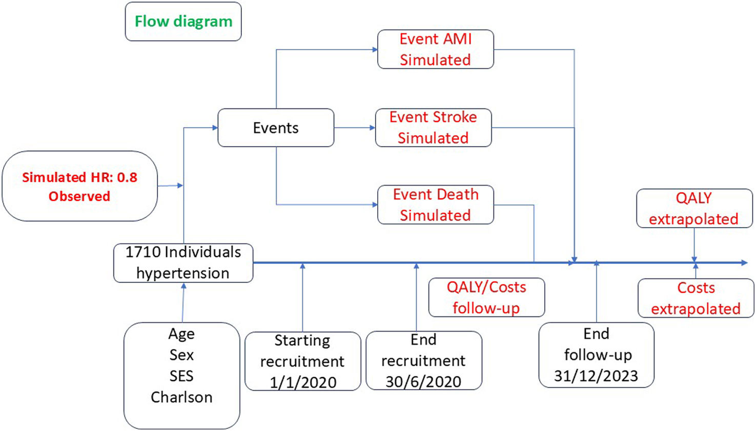
MethodDesignWe conducted a cost-utility analysis using individual patient data to compare the standard alternative (observed) with the alternative of a new treatment (simulated) by estimating quality-adjusted life years (QALY) and costs.9 This fictitious economic evaluation compared the standard- of-care (Anatomical Therapeutic Chemical [ATC] ATC code XXX1), with a new treatment (ATC code XXX2) which has not yet been used in clinical practice for individuals with conditions that increase cardiovascular risk. Our health technology assessment scenario applies once the new medicine has been authorised, but its implementation in clinical practice is still pending. We derived treatment-related risk reductions for stroke, acute myocardial infarction (AMI), and death from clinical trial in terms of hazard ratios (HR) for each event. Since our follow-up period ends on 31 March 2023, any events occurring after this date will be considered censored on the right, as the observed time is less than the event time. We estimated extrapolated QALY and costs by assuming that the subsequent trajectory will be the same as that of the equivalent population, adjusted for excess risks after stroke and AMI and sequelae due to stroke. Figure 1 show the computational workflow for estimating individual costs and QALY according to the timing of events (stroke, AMI and death).

We adopted a lifetime horizon. A 3% discount rate was applied to calculate the incremental cost and effectiveness of the treatment. The database contains information on whether each individual has experienced an event, as well as the date on which it occurred. As the results of the existing treatment are already available, we can calculate its QALY and costs directly. In contrast, we need to create a simulated alternative with results corresponding to the new treatment. The effect of the new treatment has only been taken into account during the follow-up period. Consequently, the cost of treatment is only allocated during this period. The extrapolated life expectancy is adjusted according to events that lead to death (survival 0) and those involving the costs of dependency and disutilities.
The results section provides an overview of the files in Excel and R, which are included in the Supplementary material, to help in understanding the exercise.
The Supplementary material contains additional methodological elements, such as a description of advanced methods not covered in this tutorial (SM1), probabilistic sensitivity analysis (SM2), rules for managing competitive risks in the allocation of events and survival times (SM3), elements of internal and external model validation (SM4), and the process for selecting the best model in a parametric survival analysis (SM5).
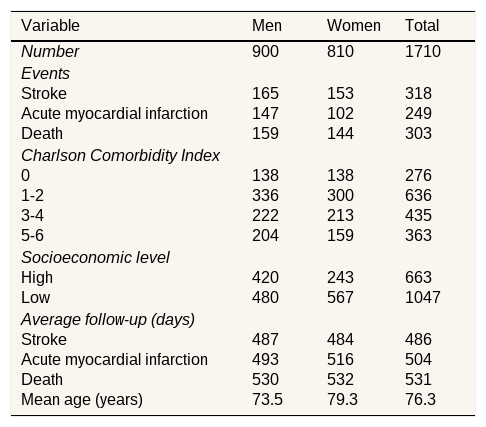
Target populationThe dataset included individuals who were diagnosed with conditions that increase cardiovascular risk and who were treated with an ATC code XXX1 drug between 1 January 2020 and 30 June 2021. These individuals were identified by their first prescription with this code. The dataset was obtained from a real-data study, but was then modified and anonymised to enable us to maintain the correlation between variables for each individual. The follow-up period for collecting data on cardiovascular events and deaths ended on 31 March 2023. These conditions included high blood pressure, high cholesterol and atrial fibrillation. Their characteristics according to sex, socioeconomic status (SES) and the Charlson comorbidity index (CCI)10 are shown in Table 1. SES was also included to analyse potential inequities. Life expectancy data are provided to estimate the long-term impact of lives saved on effectiveness. The life expectancy of survivors is assumed to be the same as that of people of the same age and sex with the excess risk of death associated to stroke and AMI.
Characteristics of the target population.
| Variable | Men | Women | Total |
|---|---|---|---|
| Number | 900 | 810 | 1710 |
| Events | |||
| Stroke | 165 | 153 | 318 |
| Acute myocardial infarction | 147 | 102 | 249 |
| Death | 159 | 144 | 303 |
| Charlson Comorbidity Index | |||
| 0 | 138 | 138 | 276 |
| 1-2 | 336 | 300 | 636 |
| 3-4 | 222 | 213 | 435 |
| 5-6 | 204 | 159 | 363 |
| Socioeconomic level | |||
| High | 420 | 243 | 663 |
| Low | 480 | 567 | 1047 |
| Average follow-up (days) | |||
| Stroke | 487 | 484 | 486 |
| Acute myocardial infarction | 493 | 516 | 504 |
| Death | 530 | 532 | 531 |
| Mean age (years) | 73.5 | 79.3 | 76.3 |
The societal perspective was employed by including both healthcare and social costs related to dependency. The standard treatment (ATC XXX1) costs €1,200 per year. New drug treatment (ATC XXX2) costs €2,500 per year. Both treatments were administered until the end of the follow-up period. Hospital costs for stroke vary according to length of stay, averaging €5,017, with a standard deviation of €2,050. For AMI, the average is €6,183, with a standard deviation of €2,364. Fifty percent of stroke patients have disabling conditions requiring treatment, resulting in formal annual social costs of €12,000 until death. Given that the level of autonomy of stroke patients is not recorded, determining which patients will experience sequelae is not possible. Therefore, we allocate €6,000 per year to all stroke cases.
EffectivenessAs the treatment in question is not yet in clinical use, we drew information regarding its effectiveness from published clinical trials. For the purposes of our analysis, we will assume that these trials indicate an HR of 0.8 for all three events. In terms of survival, stroke and AMI events carry a competing risk of death. The key intermediate measure required for estimating QALY is the time taken to reach the three events (stroke, AMI and death) with the new and standard treatment alternatives. The times for the standard alternative are already known from the observed dataset. The challenge lies in estimating the times in the new alternative via a simulated dataset. To achieve this goal, it is necessary to estimate the times to three events —stroke, AMI and death— in the alternative scenario in which the new treatment has been implemented.
Given that the risk of complications and death depends on age, the impact of the two treatment alternatives must be assessed for each patient individually and extrapolated over their life expectancy. Quality of life in terms of utility values is disaggregated by decade, SES and sex and taken from the EuroQol-5D-3 L included in the 2012 National Health Survey (Table in Excel file).11–13 The patients’ disutility was 0.1786 after a stroke and 0.0365 after AMI.11
The remaining life expectancy was calculated for each individual with one parametric survival function for men and another for women based on year-by-year mortality rates obtained, from the National Statistics Institute (INE) tables for 2019 (Table SM1 in Supplementary material) following the procedure described by Arrospide et al.14. The life expectancies were validated with the expected survival values estimated by the INE in 2019 (see Table SM5 in Supplementary material). Life expectancy was adjusted for each individual by including a HR if they had suffered a stroke (men=1.6; women=1.2)15 or an AMI (men=2.0; women=2.0).16 Individuals who died had zero life expectancy. To avoid stochastic uncertainty, the same random parameter included in the function was assigned to each individual in both alternatives. This approach explicitly adjusts for comorbidities by integrating excess mortality risk into the survival function and was previously used in a cost-effectiveness analysis of a COVID-19 vaccination programme.17
Compliance with ethical standardsThis study was performed in line with the principles of the Declaration of Helsinki and received approval on May 12, 2021 from the Ethics and Clinical Research Committee of Euskadi (study code PI2021085) which waived the informed consent as all data were anonymized.
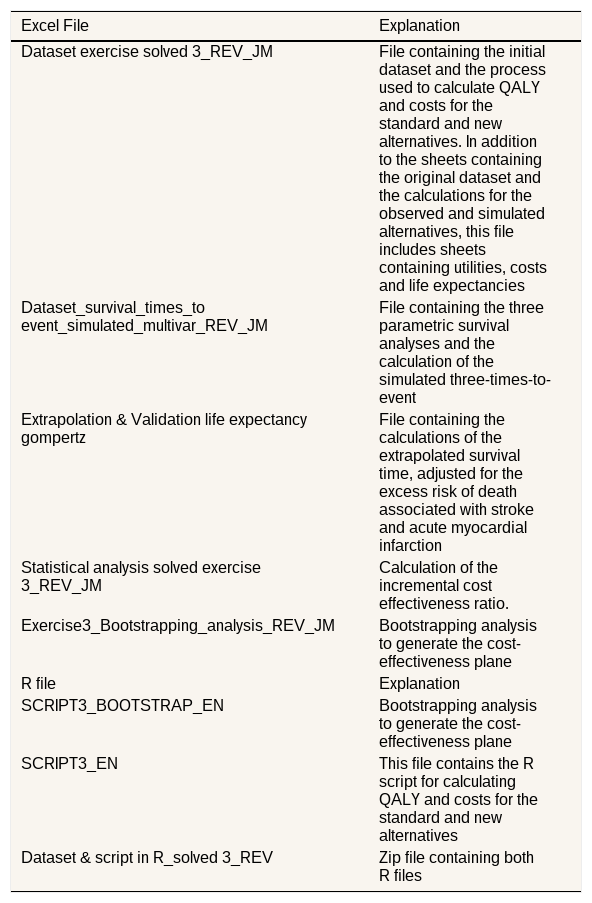
ResultsFiles in Excel and R containing the solutionThe exercise files in Excel and R (see Supplementary Material) are available in the OSF repository (https://osf.io/gyuq9/overview?view_only=748bc600f59646f1b144e21458c50a42). The description of the files can be found in Table 2.
Description of the Excel and R files used to reproduce the exercise. The files are available at https://osf.io/gyuq9/overview?view_only=748bc600f59646f1b144e21458c50a42.
| Excel File | Explanation |
|---|---|
| Dataset exercise solved 3_REV_JM | File containing the initial dataset and the process used to calculate QALY and costs for the standard and new alternatives. In addition to the sheets containing the original dataset and the calculations for the observed and simulated alternatives, this file includes sheets containing utilities, costs and life expectancies |
| Dataset_survival_times_to event_simulated_multivar_REV_JM | File containing the three parametric survival analyses and the calculation of the simulated three-times-to-event |
| Extrapolation & Validation life expectancy gompertz | File containing the calculations of the extrapolated survival time, adjusted for the excess risk of death associated with stroke and acute myocardial infarction |
| Statistical analysis solved exercise 3_REV_JM | Calculation of the incremental cost effectiveness ratio. |
| Exercise3_Bootstrapping_analysis_REV_JM | Bootstrapping analysis to generate the cost-effectiveness plane |
| R file | Explanation |
| SCRIPT3_BOOTSTRAP_EN | Bootstrapping analysis to generate the cost-effectiveness plane |
| SCRIPT3_EN | This file contains the R script for calculating QALY and costs for the standard and new alternatives |
| Dataset & script in R_solved 3_REV | Zip file containing both R files |
The electronic medical records for the 1710 participants provided the following variables: treatment group: standard treatment; age: age; sex; SES: low/high as defined by the copayment category); work activity: pensioner/worker; Charlson_factor: CCI; stroke event: yes/no; AMI event: yes/no; death event: yes/no; cost of hospitalization from analytical accounting (variable Coste_proc); time to stroke event (Follow-up_stroke): time from start of treatment to stroke event or end of follow-up if no event; time to AMI event (Follow-up_AMI): time from start of treatment to AMI event or end of follow-up if no event; time to death event (Follow-up_death): time from start of treatment to death event or end of follow-up if no event; time to total follow-up (Total_follow-up): time from the start of treatment to the end of the study follow-up. If the patient has no events, these four times are equal. The time until each event is shown in days.
We derived utilities disaggregated by sex and SES from the 2012 Spanish Health Survey.11 The table shows the utilities per decade and, for each life expectancy, calculates the average utility according to how long a person will remain in each decade.
Calculating the new times to event in the simulated alternativeThe follow-up period ends on 31 March 2023 for patients who are still alive, or on the date of their death. The estimated times to event, as calculated by the parametric functions, were converted into final times to event in the simulated dataset according to the established rules for addressing competing risks. These rules are fully described in the Supplementary Material. The simulated time to death is the estimated time if it is shorter than the final observed time for each individual. Conversely, the simulated time is the same as the observed time. For both stroke and AMI, an event is deemed to have occurred if the estimated time is shorter than the end of the follow-up period. This function also enabled the HR of each event with the new treatment (HR=0.8) to be included. The ‘Dataset_survival_times_to_event_simulated’ file displays the survival analyses and estimated event times. Assuming the same HR for all three events is unrealistic, but this simplified exercise is intended to facilitate reproduction.
The only change made to the observed dataset to create the simulated dataset was the substitution of events and times until the event, achieved by applying the rules to address the competing nature of the values estimated by the parametric functions. Therefore, as they depend on events, the QALY and costs also change. The cost of treatment also changes to account for the new drug.
Parametric survival analysisFirst, we analysed the time to each event for the population treated with the conventional drug using parametric survival models including as covariates age, sex and CCI. This enables us to select three age-adjusted survival functions depending on the lowest Akaike information criterion (AIC) value. Second, we apply inverse Gompertz (death) and Weibull (stroke and AMI) functions to estimate the adjusted time to event in the simulated dataset. To achieve this, we solve the inverse function of the standard probability survival function with time to event as the outcome variable. Caro et al.6 presented formulas for these ‘quantile functions’ on page 115 of their book. A random parameter is added to incorporate first-order or stochastic uncertainty.18 The second step is to calculate the times to event for the simulated alternative, incorporating the HR into the function.
The formulas are provided in Excel and R files. Caro et al.6 described the combination of inputs and equations from different sources as incorporating external data on intervention effects.
Steps to calculate QALY for each individual in the observed datasetLife expectancy is assigned according to age, sex, and CCI and calculated in the file “Validacion supervivencia Gompertz” (using the Life_expectancy variable).
Life expectancy is adjusted by discounting via the continuous formula (Disc_Life_Expectancy variable). Cases of death have a value of 0 in this variable and are assigned by filtering.
To assign utilities to individuals according to their age, we must consider that the utility differs for each decade. According to age, life expectancy and the utilities for each decade according to sex, the average utility by age and sex is calculated in the life expectancy sheet (Utility_Table).
To make the calculations easier to understand, the following distinction is made:
QALYs_disc_Extrap: post-follow-up or extrapolated QALYs. Discount-adjusted QALY (the ‘QALY_disc’ variable) are calculated by multiplying the ‘Disc_Life_Spe_disc’ variable by the mean utility for each age, taken from the ‘Utility_Table’. For the deceased, a value of 0 QALYs is assigned.
QALYs_disc_follow-up is the number of QALY to be calculated during the follow-up of the study. This accounts for the period before and after the stroke, as disutility needs to be applied after the stroke. These QALYs are not discounted, as the periods have already occurred19.
Finally, both QALY are summed to yield the total QALY (QALY_total).
Steps to calculate the cost for each individual in the observed datasetWe distinguish between three types of cost:
- •
Treatment costs (Cost_tratam): these costs are calculated by multiplying the adjusted life expectancy+the duration of follow-up during the study by the cost of treatment according to group.
- •
Costs of stroke sequelae (Cost_dependency): the poststroke follow-up duration and the discounted life expectancy duration are added according to the continuous formula (variable Disc_Espe_life) and multiplied by the annual sequelae cost (C_stroke_sequelae). A cost of 0 is assigned to deceased patients.
- •
Hospital cost of events (Coste_hospital_eventos): add the costs of stroke and AMI with no discount.
Finally, the three costs are added together (variable Total_cost_disc).
Steps to calculate costs and QALYs in the simulated dataset for each individualOnce the QALY and costs have been calculated in the observed dataset, the dataset is modified to estimate the QALYs and costs in the simulated dataset. To achieve this, the times to event are simply changed according to the previously described procedure. Once the times have changed, the event assignments are recalculated. Each case is analysed separately according to the rules described to deal the competing risks.
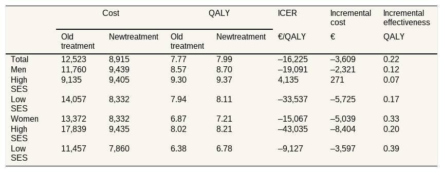
Statistical analysis of the pooled databaseThe dataset is analysed by calculating the incremental cost-effectiveness ratio (ICER) according to group, sex, and SES (Table 3). To achieve this, the two datasets (observed and simulated) are combined in a single file by adding the treatment variable. The results are shown in the Statistical Analysis Solved Exercise 3 file, which contains the ICER calculation disaggregated by sex and SES, as well as the cost-effectiveness plane. These quantitative results are purely fictitious and are provided to demonstrate how to complete the exercise using both Excel and R.
Results of cost-utility analysis of old (ATCXXX1) versus new (ATCXXX2) treatment).
| Cost | QALY | ICER | Incremental cost | Incremental effectiveness | |||
|---|---|---|---|---|---|---|---|
| Old treatment | Newtreatment | Old treatment | Newtreatment | €/QALY | € | QALY | |
| Total | 12,523 | 8,915 | 7.77 | 7.99 | –16,225 | –3,609 | 0.22 |
| Men | 11,760 | 9,439 | 8.57 | 8.70 | –19,091 | –2,321 | 0.12 |
| High SES | 9,135 | 9,405 | 9.30 | 9.37 | 4,135 | 271 | 0.07 |
| Low SES | 14,057 | 8,332 | 7.94 | 8.11 | –33,537 | –5,725 | 0.17 |
| Women | 13,372 | 8,332 | 6.87 | 7.21 | –15,067 | –5,039 | 0.33 |
| High SES | 17,839 | 9,435 | 8.02 | 8.21 | –43,035 | –8,404 | 0.20 |
| Low SES | 11,457 | 7,860 | 6.38 | 6.78 | –9,127 | –3,597 | 0.39 |
ICER: incremental cost-effectiveness ratio; QALY: quality-adjusted life year; SES: socioeconomic status.
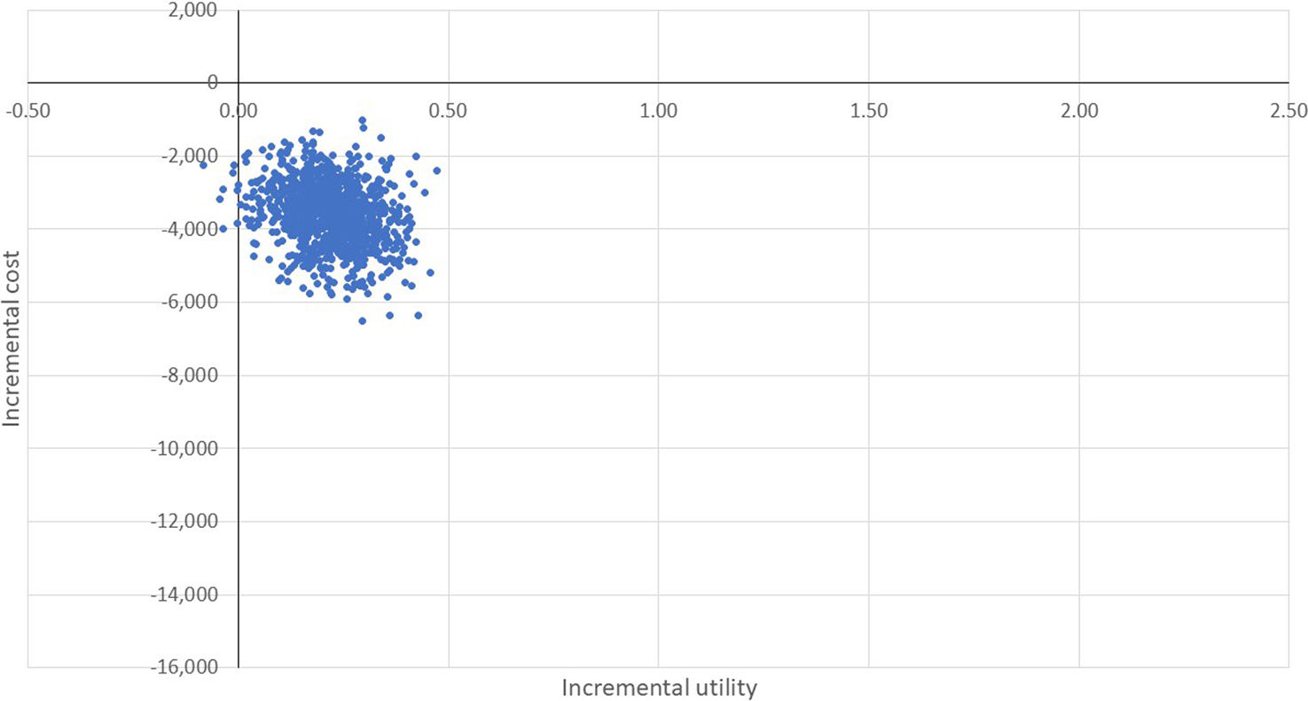
Further statistical analysis can be performed by adjusting for age, sex, SES and Charlson variables via SUR20 or separate GLM21 regression for the numerator and denominator. Glick's book21 serves as a reference, as his approach to economic evaluation in clinical trials can be applied to the resulting database. We applied bootstrapping to assess the uncertainty related to the sample.22 The cost-effectiveness plane generated through bootstrapping in the file Ejercicio_3_solucion_25_Excel_nuevo is shown in Figure 2.
Discussion
This introductory exercise illustrates how integrating RWD and DES allows real-world events to be combined with the results of a hypothetical clinical trial, thereby streamlining the process of economic evaluations. Registries integrate clinical databases from EHR containing diagnoses coded via the International Classification of Diseases, as well as diagnostic test results, surgical procedures and pharmacological treatments. They also collect administrative databases that provide information on the population's overall use of resources. In Spain, the National Health System covers practically the entire population. Although 20% of the population also has private insurance, this does not include pharmaceutical benefits, enabling their diagnoses to be recorded. Consequently, these registries provide comprehensive data on all diseases and associated costs for the entire population. Economic evaluations based on these records can measure the efficiency of healthcare interventions for the population. Registry-based economic evaluations can accurately measure the efficiency of population-level healthcare interventions. An example of this is the cost-utility study of the SARS-CoV-2 vaccine in the Basque population, which was based on a database of 2.25 million people.17
Developing proficiency in simulation modelling is facilitated by the growing availability of technical resources and survival analysis tools. The GitHub repository offers FORECAST (FOrward REsearch on Clinical and Survival Trends), an application (https://fwdcast.github.io/) that analyses a database and estimates the best parametric survival function.23,24 Standardized tools are essential to foster the rigorous and transparent use of RWD in economic evaluations.25
We would like to emphasize that this tutorial is purely introductory in scope, and that conducting a real-world cost-effectiveness study requires advanced methods which are not described here. Consequently, this tutorial does not cover the concepts of first- and second-order uncertainty,18 competing risks,7 parametric survival functions,26 distributions for probabilistic sensitivity analysis,18 propensity scores for balancing groups,27,28 validation and calibration procedures,18 or variance-covariance matrices for Cholesky decomposition13 in functions with two correlated parameters (See Table SM1 in Supplementary material). Recently, some more advanced tutorials have been published.29–32
Availability of databases and material for replicationOpen Science Framework: A tutorial on using real-world data and discrete event simulation to conduct premarket cost-effectiveness studies of new drugs (https://osf.io/gyuq9/overview?view_only=748bc600f59646f1b144e21458c50a42). Files are available under the terms of the Creative Commons Attribution 4.0 International license (CC-BY 4.0).
Numerous studies aim to replicate clinical trial findings through electronic medical records and real-world data but their application in economic evaluation has been slow.
What does this study add to the literature?This study explains how to perform a cost-utility analysis of a new treatment for a generic disease using an introductory tutorial that combines discrete event simulation with real-world data.
What are the implications of the results?Combining discrete event simulation with real-world data streamlines the process of economic evaluation.
Isaac Aranda-Reneo.
Transparency declarationThe corresponding author, on behalf of the other authors guarantee the accuracy, transparency and honesty of the data and information contained in the study, that no relevant information has been omitted and that all discrepancies between authors have been adequately resolved and described.
Authorship contributionsJ. Mar and M. Soto-Gordoa designed the study. I. Larrañaga and V. Gimeno conducted the statistical analysis. J. Mar led the overall writing of the manuscript; I. Larrañaga and V. Gimeno wrote the first draft of the methods and results section; M. Soto-Gordoa commented on, corrected, and improved the various versions of the manuscript. M. Soto-Gordoa reviewed the literature. All authors reviewed the manuscript, providing substantial comments.
FundingNone.
Conflicts of interestNone.