


Obtaining reliable health estimates at the small area level (such as neighbourhoods) using survey data usually poses the problem of small sample sizes. To overcome this limitation, we explored smoothing techniques in order to estimate poor mental health prevalence at the neighbourhood level and analyse its profile by income in Barcelona city (Spain).
MethodA Bayesian smoothing model with a logit-normal transformation was applied to four repeated cross-sectional waves of the Barcelona health survey for 2001, 2006, 2011 and 2016. Mental health status was identified from the 12-item General Health Questionnaire. Income inequalities were analysed with neighbourhood income in quantiles for each year and trends in the pooled analysis.
ResultsThe prevalence of poor mental health ranged from 14.6% in 2001 to 18.9% in 2016. The yearly difference between neighbourhoods was 12.4% in 2001, 16.7% in 2006, 14.2% in 2011, and 20.0% in 2016. The odds ratio and 95% credible interval (95%CI) of experiencing poor mental health was 1.40 times higher (95%CI: 1.02-1.91) in less advantaged neighbourhoods than in more advantaged neighbourhoods in 2001, 1.61 times higher (95%CI: 1.01-2.59) in 2006 and 2.31 times higher (95%CI: 1.57-3.40) in 2016.
ConclusionsThis study shows that the Bayesian smoothed techniques allows detection of inequalities in health in neighbourhoods and monitoring of interventions against them. In Barcelona, mental health problems are more prevalent in low-income neighbourhoods and raised in 2016.
Obtener estimadores de salud en áreas pequeñas (como los barrios) utilizando datos de encuestas supone hacer frente al problema de insuficiente tamaño muestral. Para superar esta limitación exploramos técnicas de alisado con el fin de estimar la prevalencia de mala salud mental a nivel de barrio y analizar su patrón por renta en la ciudad de Barcelona (España).
MétodoSe aplicó un modelo de alisado bayesiano con transformación logística-normal a cuatro muestras transversales repetidas de la Encuesta de Salud de Barcelona para los años 2001, 2006, 2011 y 2016. La salud mental fue identificada con el Cuestionario General de Salud de 12-items. Las desigualdades de ingreso se analizaron por cuantiles de la renta por barrio para cada año y las tendencias en el análisis conjunto.
ResultadosLa prevalencia de mala salud mental oscila entre el 14,6% en 2001 y el 18,9% en 2016. La diferencia entre barrios fue del 12,4% en 2001, del 16,7% en 2006, del 14,2% en 2011 y del 20,0% en 2016. La odds ratio y el intervalo creíble al 95% (IC95%) de experimentar mala salud mental fue 1,4 veces superior (IC95%: 1,02-1,91) en los barrios menos aventajados respecto de los más aventajados en 2001, de 1,61 (IC95%: 1,01-2,59) en 2006 y de 2,31 (IC95%: 1,57-3,40) en 2016.
ConclusionesEste estudio muestra que las técnicas de alisado bayesiano permiten la detección de desigualdades en salud a nivel de barrios para su monitorización e intervención con el fin de reducirlas. En Barcelona, los problemas de salud mental son más prevalentes en los barrios de menor renta y se incrementaron en 2016.
Monitoring indicators at the small area level has been a growing area of research in the last few decades, allowing the detection of widening socioeconomic inequalities.1 In particular, the use of official registers has enabled identification of socioeconomic health inequalities in mortality in small areas across European and Spanish cities.2,3 Estimation of health inequalities at the small areal level is of a major interest from a policy perspective as it allows improvement and monitoring of community health interventions. Interest in this topic has increased since the economic crisis of 2008, with systematic reviews reporting worsening in a variety of health outcomes and especially in mental health trends.4,5 In Spain, since the 2008 economic crisis, mental health has clearly deteriorated especially among men in the lowest socioeconomic position and the long-term unemployed.6 Previous evidence indicates that the urban environment is associated with worse mental health, although identification of a causal link is hampered by the complex interactions between urban environments and individual characteristics.7–9 However, there is scarce evidence of trends in inequalities at the small area level using survey data. Administrative delimitation of small areas does not generally respect an even distribution of population sizes so these small areas, as neighbourhoods, can register too few cases than statistically recommended10. In this case, indirect estimates for small areas can be obtained with spatial information under the principle that “the closer, the more similar”.11 Information from contiguous areas can be borrowed to smooth the estimate, so that a higher weight is assigned to the estimate of the closest areas, decreasing the problem of small sample size. The most common practice is to use random area effects to account for between-area variation.12
When smoothing techniques are used from surveys, small area estimation has to deal with missing values, and take into account the sampling design used in the estimates. Fortunately, recent approaches based on Bayesian smoothing techniques have been developed to account for sampling design.13,14 Any model that does not take sampling weights into account will be rendered biased. In the case of binary outcomes, sampling weights can be incorporated into the model by several possible transformations of the (binary health) outcome variable.14 In this study, we used the logit-normal transformation to obtain smoothed estimates of mental health at the neighbourhood level. Our investigation extends previous work on small area estimation using survey data in Spain by incorporating for the first time a complex survey design into small area estimation.15
We restricted our analysis to Barcelona city. The city lies in the North-East coast of Spain and has 1.7 million inhabitants. To our knowledge, it is the only city in Spain with data on mental health obtained regularly every 5 years between 2001 and 2016 through the Barcelona Health Survey (BHS). The BHS collects information from a representative sample of each of the 10 administrative districts of the city but not for the 73 neighbourhoods. These neighbourhoods group populations of unequal size, the largest with a population around 60 000 and the smallest with 500, with sharp socioeconomic differences.16
The objective of this study was, first, to estimate the prevalences of poor mental health in Barcelona at the neighbourhood level from 2001 to 2016 and, second, to analyse the association of mental health with neighbourhood income and its trend during this period.
MethodPopulation and variablesData were drawn from the 5-yearly BHS for 2001, 2006, 2011 and 2016. The BHS sample design consists of random selection of the population from the official register stratified by district according to age and sex quotas. Non-respondents were substituted by the population of the same sex and age group until the target sample was reached. Interviews were conducted face-to-face by trained professionals with computer-assisted personal interviewing. The sample size was computed to achieve a precision of ±2% for the whole city and ±6% for the 10 districts.
Mental health was measured with the 12-item version of the General Health Questionnaire (GHQ-12). The questionnaire focuses on the risk of mental disorders, occurring in the last 30 days, and is a widely used screening instrument to detect risk of current, diagnosable psychiatric disorders. It has been shown to be a valid and reliable screening tool for the Spanish population.17 The twelve questions were answered on a 4-point Likert scale (from 1 to 4). Following recommendations, we used a 2-point scoring method, rating a problem as absent (1 or 2) or present (3 or 4). Participants scoring 3 or more current problems were classified as having poor mental health.18
Neighbourhood income level for 2016 was taken from estimated official reports consisting of a disposable family income index imputed through a set of economic neighbourhood dimensions.16 To avoid confusion from income variations by year, all computations were performed with income from 2016. Quintiles were introduced from the most advantaged (as the reference category in the interval of 119-214.7, where 100 stands for the mean income of the city) to the least advantaged (from 49.9 to 72.5). A sensitivity analysis was performed with yearly income.
To improve the estimates, we included the centred distributions of age and sex of the neighbourhood as a sociodemographic variable.
Statistical model for smoothed estimatesFirst, normalised post-stratification weights were computed through the official population register by age and sex for each neighbourhood. The correction of the sampling weights aimed to make the distribution of the sample across neighbourhoods as similar as possible to the population. The direct estimates of poor mental health by area k, corrected with post-stratification weights (Pk,) are asymptotic estimators of the true area prevalences, but it is not guaranteed that the probability be constrained in the interval (0,1), in particular in areas with small sample size. To overcome this limitation, a convenient logit-normal transformation consists of defining the total counts of poor mental health of area k, yk, as the logistic of Pk or logit(Pk).13 The interested reader can found further statistical details in the Supplementary Material Appendix. In this way, the sampling design is incorporated into the estimation. To smooth the prevalences with information from the neighbourhood areas, we use Bayesian hierarchical models. In particular, we use the model proposed by Besag-York-Mollie19 (BYM) which takes in to account two types of random effects: spatial (uk) and heterogenous (vk). Accordingly, the logit(Pk) can be modelled as the linear combination of these two random effects as:
where XEk stands for (centred) area average age and Xsk for the (centred) proportion of women at the area level. These covariates were introduced to obtain better estimates and meaningful fitted and posterior distributions for the intercept and its 95% Credibility Intervals (95%CI). Subscripts in equation (1) indicating yearly computations were omitted for simplicity. Prior distributions are assigned to the random effects, and hyper prior distributions to the parameters of the prior distributions. The structural spatial residual is modelled as an intrinsic conditional autoregressive structure (iCAR) whose precision matrix (the inverse of the variance–covariance matrix) is proportional to the adjacent neighbourhoods. The heterogenous effect is assumed to have a normal distribution with mean 0 and variance σu. A uniform distribution U(0,∞) was assigned to the standard deviations of both random effects specified in the BYM. A normal vague prior distribution was assigned to the parameters of the intercept and coefficients. The model is scaled in the spatial variance in order to unify the interpretation of the prior and make the results transferable between applications.
Unlike other possible transformations apart from the logit-normal transformation, a different approach is the effective sample size method. Briefly, the method consists of computing the effective sample (mk*) as the sample size that is needed to match the variance from a random sample with that under a complex sample design. Therefore, the effective sample size, rather than the actual sample size, acknowledges the variable information that each individual supply under complex sampling.13,20 Accordingly, the effective number of cases can be computed as yk*=mk*·Pk. In this paper, we show smoothed prevalence estimates applying the logit-normal transformation and used the effective sample method as a sensitivity analysis.
Statistical model for the association of income and trend with poor mental healthTo analyse the association of mental health with neighbourhood income for each year, we simply added to equation (1) the quintiles of neighbourhood income IQk introduced as dummy variables with the reference category as the most advantaged neighbourhood (in bold the vector of coefficients) according to:
where the subscript for time is omitted for simplicity.
To assess the profile of inequalities in mental health by income, we used a spatio-temporal model with the pooled data across years. The temporal dimension is introduced with a common trend and random area effects to allow for deviations from trend in equation (2). An interaction term with time trend, as a continuous variable, and the neighbourhood income accounts for deviations from trend by income quantiles, and the complete specification follows the expression:
where β4 stands for the coefficient of the common trend, dk stands for the area random effect assumed to be distribute as a Normal (0, σd) and β5 the interaction term between income and time. Analogous to the first model, a uniform distribution U (0,∞) is assigned to the standard deviations of the random effects (including that of time) and a normal vague prior distribution to the parameters of the intercept and coefficients. The model is also scaled in the spatial variance. We report selection model measures: the Akaike information criteria (AIC), the deviance information criteria and the conditional predictive ordinate, with smaller values meaning better fit. Other possible specifications of time that relax the linearity hypothesis in (3) consists of also smoothing time dynamically with the prior and or subsequent observation and even its interaction with the spatial and random terms. We assessed the performance of some of these models with the selection model criteria but the improvement in these measures were negligible compared with our benchmark model so they were excluded (results available on request).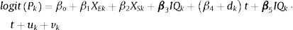
Estimation based on the classical BYM model has been criticised due to the problem of non-identifiability between the spatial random effect and the heterogeneous effect. In order to evaluate to what extent these limitations may affect the results, a sensitivity analysis has been carried out using the BYM2 model.21
To fit all models, we used the Bayesian framework with the Integrated Nested Laplace Approximation computation INLA.22 All computations were performed with R programme version 4.0.04.
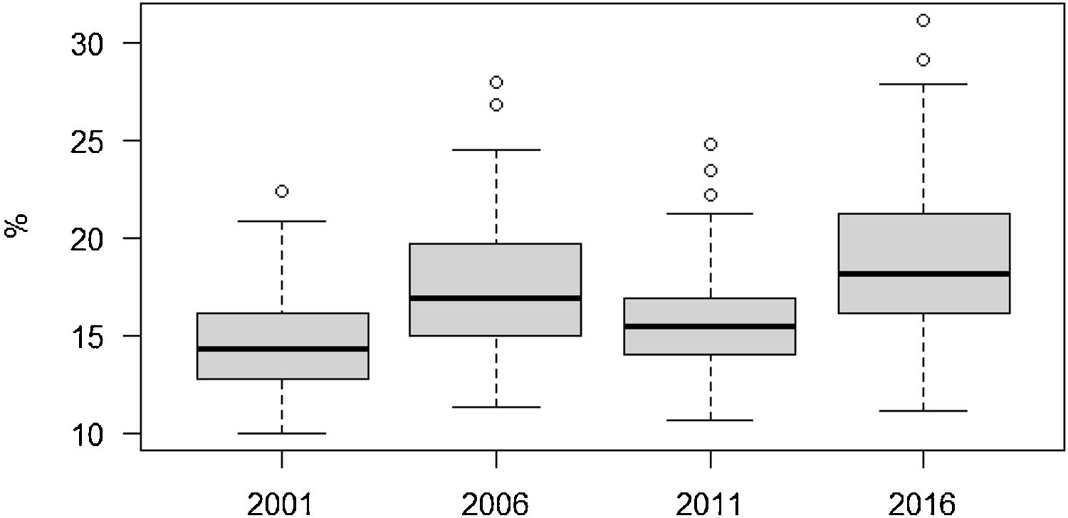
ResultsPrevalence estimates of poor mental healthDue to the sparse number cases in some areas, the direct estimates of poor mental health shown in Table 1 ranged between of 0% and 100% for each year, which is problematic. In contrast, the smoothed estimates showed a smaller range, between 9.9% and 31.1%. The reduction in the dispersion of the direct estimates are also shown in the narrower interquartile range and the reduction of the coefficient of variation in the order of between one-fifth and almost 3 times lower. The distribution was more concentrated in 2001 and 2011, although for 2001 this could be due to the larger sample size. The interquartile difference ranged from 3% in 2011 to 5.1% in 2016. The maximum difference in poor mental health between neighbourhoods was fairly constant and was greater than 12% except in 2016, when it increased: 12.4% in 2001, 16.7% in 2006, 14.2% in 2011 and 20.0% in 2016. For these years, the prevalence of poor mental health and 95%CI were 14.6% (13.1%,15.6%), 17.5% (15.3%,19.3%), 15.7% (13.6%,17.6%), and 18.9% (16.5%,20.8%), respectively.
Summary statistics for the population and dispersion measures of direct and smoothed estimates of poor mental health by year.
| 2001 | 2006 | 2011 | 2016 | |
|---|---|---|---|---|
| Population | 1,507,346 | 1,610,774 | 1,620,292 | 1,608,710 |
| Sample size | 7519 | 2405 | 3210 | 3219 |
| Poor mental health | ||||
| Total cases | 1072 | 369 | 477 | 583 |
| Smoothed prevalence (%) | 14.6 | 17.5 | 15.7 | 18.9 |
| Dispersion measures | ||||
| Total range (%) | ||||
| Direct estimates | 0-100 | 0-100 | 0-100 | 0-100 |
| Smoothed | 9.9-22.3 | 11.2-27.9 | 10.6-24.8 | 11.1-31.1 |
| Interquartile range (%) | ||||
| Direct estimates | 10.5-17.9 | 5.9-20.4 | 7.3-18.8 | 8.8-24.8 |
| Smoothed | 12.7-16.2 | 14.9-19.6 | 13.9-16.9 | 16.1-21.2 |
| Coefficient of variation | ||||
| Direct estimates | 92.2 | 84.9 | 105.5 | 60.0 |
| Smoothed | 17.1 | 19.6 | 17.9 | 21.6 |
Year-specific smoothed estimates of poor mental health with the logit-normal transformation are shown in Figure 1. Larger dispersion was observed in 2006 and 2016 with poor mental health tending to increase except in 2011 when it returned to the 2001 level. A similar profile was obtained in the sensitivity analysis with the effect size method (see Fig. I in online Appendix). No specific spatial pattern was observed for the smoothed estimates before the economic crisis of 2008, but for 2011 and 2016 worse mental health tended to persist in the low-income neighbourhoods of the north-east and south-west of the city (see Fig. II in online Appendix).
Association and trends of neighbourhood income with poor mental health
Income inequalities for the least advantaged neighbourhoods for all years, except 2011, are shown in Table 2. The odds ratio (OR) and 95%CI of experiencing poor mental health was 1.40 (95%CI: 1.02-1.91) times higher in less advantaged compared with more advantaged neighbourhoods in 2001, with OR 1.61 (95%CI: 1.01-2.59) times higher in 2006 and OR 2.31 (95%CI: 1.57-3.40) times higher in 2016 for the fifth poorer income quintile IQ5 and OR 2.10 (95%CI: 1.42-3.08) for IQ4. A visual representation of this profile of income inequalities is reported in Fig. III in online Appendix, where a steeper gradient was observed in 2006 and 2016.
Odds ratios and 95% credible intervals of poor mental health and by year and the pooled estimate.
| 2001 | 2006 | 2011 | 2016 | Pooled | |
|---|---|---|---|---|---|
| Age | 1.04 (0.99-1.09) | 1.01 (0.97-1.06) | 0.98 (0.94-1.03) | 1.00 (0.97-1.04) | 1.01 (0.99-1.03) |
| Men | Reference | Reference | Reference | Reference | Reference |
| Women | 1.64 (0.54-4.99) | 2.29 (0.96-5.68) | 1.21 (0.41-3.61) | 1.17 (0.44-3.17) | 1.57 (1.03-2.39) |
| Income | |||||
| IQ 1 | Reference | Reference | Reference | Reference | Reference |
| IQ 2 | 1.04 (0.77-1.39) | 1.03 (0.63-1.66) | 0.85 (0.55-1.33) | 1.33 (0.90-1.97) | 0.99 (0.80-1.22) |
| IQ 3 | 1.17 (0.86-1.60) | 1.29 (0.78-2.12) | 0.97 (0.61-1.53) | 1.36 (0.89-2.07) | 1.14 (0.90-1.43) |
| IQ 4 | 1.29 (0.95-1.75) | 1.33 (0.81-2.18) | 1.05 (0.64-1.68) | 2.10 (1.42-3.08)a | 1.19 (0.95-1.48) |
| IQ 5 | 1.40 (1.02-1.91)a | 1.61 (1.01-2.59)a | 1.04 (0.62-1.69) | 2.31 (1.57-3.40)a | 1.34 (1.07-1.66)a |
| Time (t) | 1.00 (0.91-1.10) | ||||
| IQ 2*t | 1.07 (0.93-1.22) | ||||
| IQ 3*t | 1.05 (0.91-1.20) | ||||
| IQ 4*t | 1.15 (1.01-1.31)a | ||||
| IQ 5*t | 1.14 (0.99-1.30) | ||||
| AIC | 92.2 | 160.1 | 150.9 | 132.6 | 571.1 |
| DIC | 94.3 | 162.6 | 154.4 | 132.8 | 553.8 |
| CPO | −3.75 | −3.33 | −3.32 | −3.53 | −5.03 |
AIC: Akaike information criteria; CPO: conditional predictive ordinate; DIC: deviance information criterion; IQ: income quantile from the most advantaged IQ1 to the least advantaged IQ5.
The issue of whether income inequalities by quartiles has narrowed or expanded with time is captured with the interaction terms between income quartiles and time in the pooled analysis in Table 2. The interaction was positive and significant for less advantaged neighbourhoods, quartile IQ4, with OR 1.15 (95%CI 1.01-1.31) and almost significant for IQ5 OR 1.14 (95%CI 0.99-1.30) but not for the other neighbourhood quartiles. However, the lower value obtained by the sum of the goodness of the fit measures of the partial (yearly) models compared to the value of the pooled model with trend indicates the poorer performance of this last model, so that a conclusion on a widening inequality gap over time should be avoided. Similar results were obtained in the sensitivity analysis considering income for each year (data not shown). The sensibility analysis applying BYM2 gave also equivalent results (Appendix) but being the interaction term in pooled analysis significant also for the IQ5.
DiscussionIn this study, we obtained small area estimates (at the neighbourhood level) for poor mental health incorporating a complex survey design through the logit-normal transformation. Smoothed estimates successfully reduced variability and provided a reliable picture of mental health inequalities. We observed inequalities in poor mental health across neighbourhoods (except for 2011), which increased in 2016.
A profile of inequalities that decreased during the economic crisis in 2011 but widened again in 2016 was also found in England.23 The decrease in inequalities during the economic crisis depended on whether the dominant response was a coping response or a stressful one.24 For instance, a pioneering study investigating the relationship between economic conditions and mortality rates during the period 1972-1991 argued that a larger proportion of the population may acquire healthier habits, such as more hours of sleep, more physical exercise, less demanding work and more time for leisure, leading to a reduction in health inequalities.25 Conversely, the Spanish labour reform of 2012 may have helped to prolong the adverse effects of the economic downturn through higher unemployment rates, worse working conditions, and greater job insecurity, leading to poor prospects for younger people and disproportionately affecting the population with a lower socioeconomic position.26
As stressed by the recent above-mentioned literature,9,27 individual determinants of mental health probably have stronger mechanisms than neighbourhood settings. However, the relentless effects of the economic crisis of 2008 have exacerbated divergence in neighbourhood vulnerability. It has been suggested that mechanisms of divergence may be greater in countries, such as in Spain, with a higher proportion of home-ownership and with a tight rental housing market. In this situation, it is more difficult for low- to middle-income groups and first home buyers to obtain a mortgage than in the past, while the financial effort of renting increases, so that this population is forced to move to more deprived areas.28 In particular, evictions have been a major problem in Barcelona. From the first registers in 2013 to 2016, 12,333 evictions have been recorded, which may have contributed to increasing inequalities in the 2016 wave, as evicted persons report poor mental health up to 6 times more frequently than the general population.29
Our result agrees with recent cross-sectional studies reporting weak evidence in showing increasing inequalities in the risk of psychosocial problems among neighbourhoods.30 Although the Neighbourhood Law was withdrawn in 2011 during the economic crisis, Barcelona has continued to carry out the municipal programme Health in the neighbourhoods aimed at reducing health inequalities. The programme reached 13,600 people among 25 of the most disadvantaged neighbourhoods in the city. Participants in these community interventions ranked mental health problems as among the first priorities needing to be tackled.31 Our study cannot be interpreted as a direct evaluation of this programme but it does provide indicators on the geographical scale in which the interventions are carried out and allows interventions to be focused on the neighbourhoods most requiring them without neglecting the importance of individual effects. Because some authors have found only weak evidence of area-based interventions to avoid the adverse “neighbourhood effect” on mental health,32–34 a mix of individual-level targeted and area policy is likely to be needed.
As stated, the association observed cannot be interpreted as causal, due to the repeated cross-sectional design rather than longitudinal or instrumental variable techniques, and to the lack of a proper measure of the neighbourhood environment. A limitation of our estimated models to further explore is the potential confounding between fixed and random effects. Spatial confounding occurs when covariates have a spatial pattern and are collinear with spatial random effects. To overcome this problem, it is proposed to specify random effects as orthogonal to fixed effects.35 However, while adding spatially correlated random effects does not adjust the fixed effects for the missing covariates, it does smooth the fitted values. Another limitation of our study is that we were unable to stratify by sex due to the small sample size in some areas. In the context of this small sample size, the results should be interpreted with caution if the adjacent neighbourhoods differ in their socioeconomic and environmental settings. In this case, the smoothed estimates could deviate from real values.
Availability of databases and material for replicationData available to persons on request to xbartoll@aspb.cat from the Institut d’Investigació Biomèdica Sant Pau, Barcelona (Spain), in accordance with the data policy applicable to the Barcelona health survey.
Statistical codes to the Bayesian estimates are provided in the online Appendix.
Bayesian smoothing techniques can provide reliable estimates of the prevalence of poor mental health at the small area level. Common challenges to obtaining reliable estimates from health surveys are low sample sizes in small areas and complex designs
What does this study add to the literature?The smoothed estimates substantially reduced variability compared with direct estimates and allowed detection of socioeconomic inequalities between neighbourhoods that remained during the study period with some oscillations
What are the implications of the results?Territorial inequalities can be monitored with survey data in a small sample context. A deepening of individual-level and area-based targeted interventions are recommended to reduce these inequalities.
Miguel Ángel Negrín Hernández.
Transparency declarationThe corresponding author on behalf of the other authors guarantee the accuracy, transparency and honesty of the data and information contained in the study, that no relevant information has been omitted and that all discrepancies between authors have been adequately resolved and described.
Authorship contributionsX. Bartoll-Roca and M. Marí-Dell’Olmo contributed to the planning, conception, design and implementation of the study. M. Marí-Dell’Olmo contributed to the finalisation and analysis of the data. X. Bartoll-Roca drafted the manuscript. M. Marí-Dell’Olmo, M. Gotsens and Laia Palència contributed to methodological revision of the manuscript. K. Pérez and E. Díez contributed to critical discussion, and C. Borrell to comments on the neighbourhood environment and to the final version of the manuscript.
FundingNone.
Conflicts of interestNone.